This is the second part in my series on the "travelling salesman problem" (TSP). Part one covered defining the TSP and utility code that will be used for the various optimisation algorithms I shall discuss.
solution landscapes
If we are using evolutionary optimisation methods a solution landscape will often be referred to as a fitness landscape.
hill-climbing
Hill-climbing, pretty much the simplest of the stochastic optimisation methods, works like this:
- pick a place to start
- take any step that goes "uphill"
- if there are no more uphill steps, stop; otherwise carry on taking uphill steps
The "biggest" hill in the solution landscape is known as the global maximum. The top of any other hill is known as a local maximum (it's the highest point in the local area). Standard hill-climbing will tend to get stuck at the top of a local maximum, so we can modify our algorithm to restart the hill-climb if need be. This will help hill-climbing find better hills to climb - though it's still a random search of the initial starting points.
objective and initialisation functions
To get started with the hill-climbing code we need two functions:
- an initialisation function - that will return a random solution
- an objective function - that will tell us how "good" a solution is
For the TSP the initialisation function will just return a tour of the correct length that has the cities arranged in a random order.
The objective function will return the negated length of a tour/solution. We do this because we want to maximise the objective function, whilst at the same time minimise the tour length.
As the hill-climbing code won't know specifically about the TSP we need to ensure that the initialisation function takes no arguments and returns a tour of the correct length and the objective function takes one argument (the solution) and returns the negated length.
So assuming we have our city co-ordinates in a variable coords and our distance matrix in matrix we can define the objective function and initialisation functions as follows:
def init_random_tour(tour_length):
   tour=range(tour_length)
   random.shuffle(tour)
   return tour

init_function=lambda: init_random_tour(len(coords))
objective_function=lambda tour: -tour_length(matrix,tour) #note negation
Relying on closures to let us associate len(coords) with the init_random_tour function and matrix with the tour_length function. The end result is two function init_function and objective_function that are suitable for use in the hill-climbing function.
the basic hill-climb
The basic hill-climb looks like this in Python:
def hillclimb(
    init_function,
    move_operator,
    objective_function,
    max_evaluations):
    '''
    hillclimb until either max_evaluations
    is reached or we are at a local optima
    '''
    best=init_function()
    best_score=objective_function(best)

    num_evaluations=1

    while num_evaluations < max_evaluations:
        # examine moves around our current position
        move_made=False
        for next in move_operator(best):
            if num_evaluations >= max_evaluations:
                break

            # see if this move is better than the current
            next_score=objective_function(next)
            num_evaluations+=1
            if next_score > best_score:
                best=next
                best_score=next_score
                move_made=True
                break # depth first search

        if not move_made:
            break # we couldn't find a better move
                     # (must be at a local maximum)

    return (num_evaluations,best_score,best)
(I've removed some logging statements for clarity)
The parameters are as follow:
- init_function - the function used to create our initial solution
- move_operator - the function we use to iterate over all possible "moves" for a given solution (for the TSP this will be reversed_sections or swapped_cities)
- objective_function - used to assign a numerical score to a solution - how "good" the solution is (as defined above for the TSP)
- max_evaluations - used to limit how much search we will perform (how many times we'll call the objective_function)
hill-climb with random restart
With a random restart we get something like:
def hillclimb_and_restart(
    init_function,
    move_operator,
    objective_function,
    max_evaluations):
    '''
    repeatedly hillclimb until max_evaluations is reached
    '''
    best=None
    best_score=0

    num_evaluations=0
    while num_evaluations < max_evaluations:
        remaining_evaluations=max_evaluations-num_evaluations

        evaluated,score,found=hillclimb(
            init_function,
            move_operator,
            objective_function,
            remaining_evaluations)

        num_evaluations+=evaluated
        if score > best_score or best is None:
            best_score=score
            best=found

    return (num_evaluations,best_score,best)
The parameters match those of the hillclimb function.
This function simply calls hillclimb repeatedly until we have hit the limit specified by max_evaluations, whereas hillclimb on it's own will not necessarily use all of the evaluations assigned to it.
results
Running the two different move operators (reversed_sections and swapped_cities - see part one for their definitions) on a 100 city tour produced some interesting differences.
| reversed_sections | swapped_cities |
|---|---|
| -4039.86 | -6451.12 |
| -4075.04 | -6710.48 |
| -4170.41 | -6818.04 |
| -4178.59 | -6830.57 |
| -4199.94 | -6831.48 |
| -4209.69 | -7216.22 |
| -4217.59 | -7357.70 |
| -4222.46 | -7603.30 |
| -4243.78 | -7657.69 |
| -4294.93 | -7750.79 |
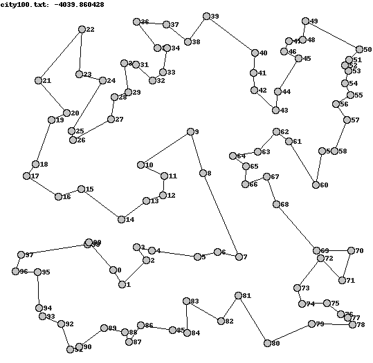
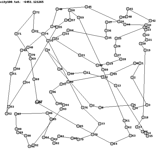
It's pretty clear then that reversed_sections is the better move operator. This is most likely due to it being less "destructive" than swapped_cities, as it preserves entire sections of a route, yet still affects the ordering of multiple cities in one go.
conclusion
As can be seen hill-climbing is a very simple algorithm that can produce good results - provided one uses the right move operator.
However it is not without it's drawbacks and is prone to getting stuck at the top of "local maximums".
Most of the other algorithms I will discuss later attempt to counter this weakness in hill-climbing. The next algorithm I will discuss (simulated annealing) is actually a pretty simple modification of hill-climbing, but gives us a much better chance at finding the global maximum for a given solution landscape.
source-code
Full source-code is available here as a .tar.gz file. Again some unit tests are included, which can be run using nosetests.
(The source-code contains more code than shown here, to handle parsing parameters passed to the program etc. I've not discussed this extra code here simply to save space.)