Psychic Origami

This is the third part in my series on the “travelling salesman problem” (TSP). Part one covered defining the TSP and utility code that will be used for the various optimisation algorithms I shall discuss. Part two covered “hill-climbing” (the simplest stochastic optimisation method).

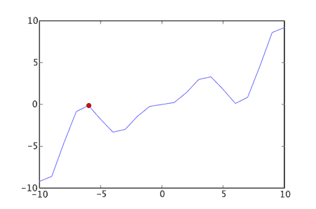
getting stuck, because you’re greedy

As I discussed in the article about hill-climbing it is possible for an algorithm to find a solution that is “locally optimal”, but not necessarily “globally optimal”. That is to say we may find ourselves with a solution that is at the top of a local maximum – it’s the best thing nearby, but it might not be the best thing. This happens with hill-climbing, because when we are offered the choice between two solutions we always take the best solution. The algorithm is “greedy”. It’s also short sighted.

So instead we could try occasionally choosing something that’s worse. By doing that the algorithm can go “downhill” sometimes and hopefully reach new areas of the solution landscape.

simulated annealing

Taking it’s name from a metallurgic process, simulated annealing is essentially hill-climbing, but with the ability to go downhill (sometimes).

It introduces a “temperature” variable. When the “temperature” is high a worse solution will have a higher chance of being chosen. It work’s like this:

1. pick an initial solution
2. set an initial temperature
3. choose the next neighbour of the current solution:
   • if the neighbour is “better” make that neighbour the current solution
   • if the neighbour is “worse”, probabilistically make this neighbour the current solution, based on the current temperature and how much “worse” the neighbour is
4. decrease the temperature slightly
5. go to 3.

By slowly cooling the temperature we become less likely to choose worse solutions over time. Initially we are able to make some pretty big jumps around the solution landscape. By the end of a run we’ll be jumping around less and less. In fact if we lower the temperature enough we end up with plain old hill-climbing.

probabilistically choosing a neighbour

Below is the Python code to decide if what probability we will assign to moving from a solution with a score of prev_score to a solution with a value of next_score at the current temperature.

def P(prev_score,next_score,temperature):
    if next_score > prev_score:
        return 1.0
    else:
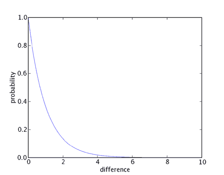
        return math.exp( -abs(next_score-prev_score)/temperature )

To keep later logic simpler I’m returning 1.0 if next_score is better – so we’ll always choose better solutions.

When the prev_score is worse we create a probability based on the difference between prev_score and next_score scaled by the current temperature. If we chart the probabilities versus the difference in scores we get (with a temperature of 1.0):

As can be seen, for small differences (relative to the current temperature) we will have a high probability. This then tails off very quickly, so solutions that are much worse are increasingly less likely to be chosen.

The net-effect being that solutions that are only a little bit worse are still fairly likely to be chosen. Much worse solutions may still be chosen, but it’s much less likely.

the cooling schedule

Temperature is a key part of simulated annealing. How we lower the temperature over time is therefore very important. There are a couple of possible approaches, but I’ll show the one outlined by Kirkpatrick et al:

def kirkpatrick_cooling(start_temp,alpha):
    T=start_temp
    while True:
        yield T
        T=alpha*T

This is a generator function that takes an initial start temperature (start_temp) and returns a series of temperatures that are alpha times the size, where alpha is less than one. So we end up with a temperature that drops off quite quickly and then slowly decreases to practically nothing.

remembering the best solution

One other minor, but key, implementation detail is saving the best solution we find during the annealing process.

During hill-climbing the current solution was always the best solution found, but simulated annealing will deliberately accept worse solutions at times. So we need to make sure we don’t just throw away the best we see. To avoid complicating the algorithm itself with extra checks of scores etc.

I am going to use a class to wrap the objective function. I’ll override the __call__ method of the class, so that I can use the instance of the class like a function – in place of the normal objective function:

class ObjectiveFunction:
    '''class to wrap an objective function and 
    keep track of the best solution evaluated'''
    def __init__(self,objective_function):
        self.objective_function=objective_function
        self.best=None
        self.best_score=None
    
    def __call__(self,solution):
        score=self.objective_function(solution)
        if self.best is None or score > self.best_score:
            self.best_score=score
            self.best=solution
        return score

We can then access then best and best_score fields when we have finished our annealing.

simulated annealing itself

The code below represents the simulated annealing algorithm. In many respects it is pretty similar to hill-climbing, but we are also concerned with a current temperature and we have introduced a probabilistic element to choosing the next solution.

def anneal(init_function,move_operator,objective_function,max_evaluations,start_temp,alpha):
    
    # wrap the objective function (so we record the best)
    objective_function=ObjectiveFunction(objective_function)
    
    current=init_function()
    current_score=objective_function(current)
    num_evaluations=1
    
    cooling_schedule=kirkpatrick_cooling(start_temp,alpha)
    
    for temperature in cooling_schedule:
        done = False
        # examine moves around our current position
        for next in move_operator(current):
            if num_evaluations >= max_evaluations:
                done=True
                break
            
            next_score=objective_function(next)
            num_evaluations+=1
            
            # probablistically accept this solution
            # always accepting better solutions
            p=P(current_score,next_score,temperature)
            if random.random() < p:
                current=next
                current_score=next_score
                break
        # see if completely finished
        if done: break
    
    best_score=objective_function.best_score
    best=objective_function.best

    return (num_evaluations,best_score,best)

The parameters are much the same as hill-climbing, but there are two extra specific to simulated annealing:

• init_function - the function used to create our initial solution
• move_operator - the function we use to iterate over all possible "moves" for a given solution
• objective_function - used to assign a numerical score to a solution - how "good" the solution is
• max_evaluations - used to limit how much search we will perform (how many times we'll call the objective_function)
• start_temp - the initial starting temperature for annealing
• alpha - should be less than one. controls how quickly the temperature reduces

I am also only reducing the temperature after either accepting a new solution or evaluating all neighbours without choosing any of them. This is done so that temperature will only decrease as we start accepting moves. As that will be less frequent than just evaluating moves we cooling will happen at a slower pace. If we are accepting lots of moves then this will drop the temperature quite quickly. If we are not accepting many moves the temperature will stay steadier - maintaining the likelihood of accepting other "worse" moves. That latter point is useful, as if we are starting to get stuck on a local maximum the temperature won't decrease - hopefully helping us get unstuck.

results

It made sense to compare simulated annealing with hill-climbing, to see whether simulated annealing really helps us to stop getting stuck on local maximums.

I performed 100 runs of each algorithm on my randomly generated 100 city tour, once with 50000 and once with 100000 evaluations. Both algorithms used the reversed_sections move operator. For simulated annealing I chose an initial temperature and alpha that seemed to perform well.

evaluations	algorithm	average	s.d.	worst	best
50000	hill-climbing	-4228.50	126.45	-4627.07	-3942.03
50000	annealing (start_temp=10, alpha=0.9999)	-4145.69	96.56	-4422.04	-3924.34
100000	hill-climbing	-4154.25	90.60	-4513.11	-3946.65
100000	annealing (start_temp=10, alpha=0.99995)	-4077.40	71.72	-4294.97	-3907.19

These results seem to show that simulated annealing performed better than hill-climbing. In fact it can be seen that with just 50000 evaluations, simulated annealing was able to do a slightly better job than hill-climbing with 100000 evaluations! This makes sense, as when running hill-climbing with logging turned on I could see that after about 50000 evaluations hill-climbing was getting stuck and restarting. With more evaluations available it was possible to push simulated annealing further still.

However in both cases I had to perform several test runs to find reasonable starting temperatures and alpha values to get these kind of results. It was quite easy to set these parameters wrong and get much worse results than with hill-climbing.

conclusion

Simulated annealing is a pretty reasonable improvement over hill-climbing. For a modest amount of extra code (in this cases 10's of lines) we are able to address hill-climbing's fundamental weakness (getting stuck) and yield much better results.

However by introducing two extra parameters we have shifted some of the burden in finding good solutions to ourselves. We have to tune these parameters carefully. Values that are good for one problem may not work so well for another. We end up with more "switches to flick" in the hope of making something work.

Next time around I will be discussing evolutionary algorithms, which pursue other ways to avoid getting stuck on local maximums and are also able to combine several solutions to explore new areas of the solution landscape.

source-code

Full source-code is available here as a .tar.gz file.

(The source-code contains more code than shown here, to handle parsing parameters passed to the program etc. I’ve not discussed this extra code here simply to save space.)

This entry was posted on Thursday, June 28th, 2007 at 1:16 pm and is filed under Development, Optimisation, Python, TSP. You can follow any responses to this entry through the RSS 2.0 feed. You can leave a response, or trackback from your own site.